This is a useful feature that allows you to keep data separate and organized across different sheets and files. If you want to know how to cross-reference cells between Excel spreadsheets, here’s how.
Cross Referencing Single Cells in Excel
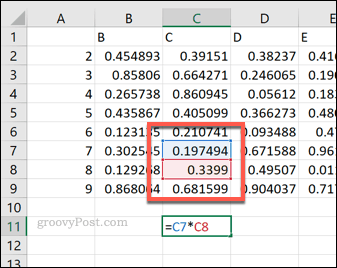
If you’ve ever used a map, you’ll be familiar with the idea of grid references. A map is split up into a grid, allowing you to pinpoint a specific location using the individual grid reference. An Excel spreadsheet works in a similar way. A spreadsheet in Excel is split into cells, which you can reference using letters for columns and numbers for rows. Cell C7, for instance, is in the cell that intersects the third column (column C) and row 7. To reference this cell in your active worksheet, type =C7 in a different cell, or use a formula containing that cell reference that combines multiple cell references together. =C7*C8 multiplies the data from C7 with the data from cell C8, for instance.
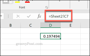
If you want to reference a cell from a different worksheet, you need to put the name of the worksheet before the cell, followed by an exclamation mark. The correct format for this is =Sheet2!C7.
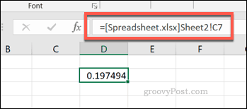
The formula =Sheet2!C7*Sheet2!C8 would multiply the data from cells C7 and C8 in a worksheet named Sheet2. You can also reference cells from another Excel spreadsheet file. You’ll need to use square brackets to identify the file, name the worksheet it’s from, then use the cell reference. For instance, =[Spreadsheet.xlsx]Sheet2!C7.
Using =[Spreadsheet.xlsx]Sheet2!C7*[Spreadsheet.xlsx]Sheet2!C8, you’d be able to multiply the data from cells C7 and C8 in worksheet Sheet2 from a file called Spreadsheet.xlsx.
Referencing Cell Ranges in Excel
It’s also possible to reference multiple cells in Excel, so long as they follow sequentially. You can use references to cell ranges in certain formulae. For instance, finding the sum of cells C7 to C10 is easy—simply type =SUM(C7:C10), using a colon to connect the start (C7) and end (C10) cells in the range.
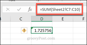
You can reference cell ranges in other worksheets and Excel spreadsheet files, too. This follows the same naming approach as listed above for individual cells. To reference a cell range from another worksheet in the same file, name the worksheet before the cell range. For instance, =SUM(Sheet2!C7:C10).
To reference a cell range from another file, use square brackets to name the file, followed by a reference to the worksheet, and finally the cell range. For example, =SUM([Spreadsheet.xlsx]Sheet2!A7:A10).
Referencing Named Cells in Microsoft Excel
Microsoft Excel allows you to give a set name to a cell, replacing the grid-style reference. To do this, select your cell, then provide a name for it in the text box next to the formula bar. You can then use this defined cell name as a reference in other cells. For example, a named cell named namedcell could be referred to in another cell as =namedcell.
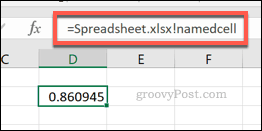
This named cell reference can be used as-is across your entire worksheet. For example, if it was on a worksheet named Sheet2, you would still use the =namedcell reference to refer to it. If you want to reference a named cell from another Excel spreadsheet, you don’t need to use square brackets. Typing =Spreadsheet.xlsx!namedcell would refer to a cell named namedcell saved in an external Excel spreadsheet file named Spreadsheet.xlsx instead.
Organizing Data in Microsoft Excel
Knowing how to cross-reference cells in Excel allows you to organize data more effectively. You don’t need to work on a single sheet—you can use data from a single cell across different worksheets and spreadsheet files. You can then take this data and refer to it in other software. For instance, you could begin embedding Excel with your OneNote notes. If you’re new to Excel, don’t worry—there are plenty of Excel tips that will help you get up to speed quickly.
![]()

